Gender Inequality

Introduction
Gender wage inequality has long been the subject of public interest. Some argue that it is due to discrimination, whereas others argue that it is due to differing years of experience (which may or may not itself be caused by discrimination in the workplace). As a woman, I am very interested in this topic - even interested enough to write a dissertation about it!
Dataset
Here, I use a small sample of 50 executives by Omega Group Plc. This is not an awfully large sample, but this gives us a useful insight nonetheless.
omega <- read_csv(here::here("data", "omega.csv"))
glimpse(omega) # examine the data frame
## Rows: 50
## Columns: 3
## $ salary <dbl> 81894, 69517, 68589, 74881, 65598, 76840, 78800, 70033, 635…
## $ gender <chr> "male", "male", "male", "male", "male", "male", "male", "ma…
## $ experience <dbl> 16, 25, 15, 33, 16, 19, 32, 34, 1, 44, 7, 14, 33, 19, 24, 3…Relationship between salary and gender?
There are different types of analysis to be conducted for on the dataset to answer the simple question: does salary differ significantly between the two genders?
Confidence interval analysis
Looking at the summary statistics of the salary received by male and female executives, the confidence intervals do not overlap, and we conclude that there is at least a 95% statistically significant difference between the mean salaries of the male and female executives.
# Summary Statistics of salary by gender
gender_summary <- mosaic::favstats (salary ~ gender, data = omega)

# Create dataframe of low and high confidence intervals
gender_dataframe <- gender_summary %>%
  select(gender, mean, sd, n) %>%
  mutate(se = sd / sqrt(n),
         t = qt(0.975, n-1),
         margin = t * se,
         l_ci = mean - margin,
         h_ci = mean + margin) %>%
  select(gender, mean, sd, n, t, se, margin, l_ci, h_ci)

# Display dataframe
gender_dataframe
## gender mean sd n t se margin l_ci h_ci
## 1 female 64543 7567 26 2.06 1484 3056 61486 67599
## 2 male 73239 7463 24 2.07 1523 3151 70088 76390Hypothesis Testing
Given the null hypothesis: salary does not differ between genders; and the alternative hypothesis: salary does differ between genders, a t-test is conducted using both the formula and the infer package. Both ways have found the t-test statistic statistically significant, and that there is evidence of difference in means of income between the genders.
# hypothesis testing using t.test()
t.test(salary ~ gender, data = omega)
##
## Welch Two Sample t-test
##
## data: salary by gender
## t = -4, df = 48, p-value = 2e-04
## alternative hypothesis: true difference in means between group female and group male is not equal to 0
## 95 percent confidence interval:
## -12973 -4420
## sample estimates:
## mean in group female mean in group male
## 64543 73239# hypothesis testing using infer package
library(infer)
# initialise and find the dataset
obs_diff_sg <- omega %>%
specify(salary ~ gender) %>%
calculate(stat = "diff in means", order = c("female", "male"))
# simulate 1000 times
omega_null <- omega %>%
specify(salary ~ gender) %>%
hypothesise(null = "independence") %>%
generate(reps = 1000, type = "permute") %>%
calculate(stat = "diff in means",
order = c("female", "male"))
# plotting observed dataset
omega_null %>% visualize() +
shade_p_value(obs_stat = obs_diff_sg, direction = "two-sided")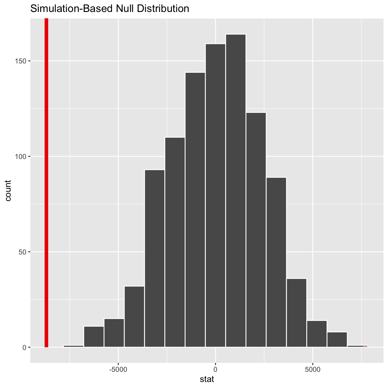
omega_null %>%
  get_p_value(obs_stat = obs_diff_sg, direction = "two_sided")
## # A tibble: 1 × 1
## p_value
## <dbl>
## 1 0Relationship between experience and gender?
Gender may not be an explanatory variable for salary, as there may be another variable, for example, educational level and/or years of work experience, that may differ systematically between the genders and hence explain the systematic underpaying of females.
Hypothesis testing
Examining such relationship using a t-test, using both formula and the infer package. There is again evidence to suggest that there is statistically significant differences in experience between genders. We may suspect that the systematic difference in experience may have an impact on the systematic difference in salary between the genders.
# t-test method
t.test(experience ~ gender,
       alternative = "two.sided",
       conf.level = 0.95,
       data = omega)
##
## Welch Two Sample t-test
##
## data: experience by gender
## t = -5, df = 43, p-value = 1e-05
## alternative hypothesis: true difference in means between group female and group male is not equal to 0
## 95 percent confidence interval:
## -19.35 -8.13
## sample estimates:
## mean in group female mean in group male
## 7.38 21.12# infer package method
# initialise based on dataset
obs_diff_eg <- omega %>%
specify(experience ~ gender) %>%
calculate(stat = "diff in means", order = c("female", "male"))
# simulate this 1000 times
experience_null <- omega %>%
specify(experience ~ gender) %>%
hypothesise(null = "independence") %>%
generate(reps = 1000, type = "permute") %>%
calculate(stat = "diff in means",
order = c("male", "female"))
# plotting observed dataset
experience_null %>% visualize() +
shade_p_value(obs_stat = obs_diff_eg, direction = "two-sided")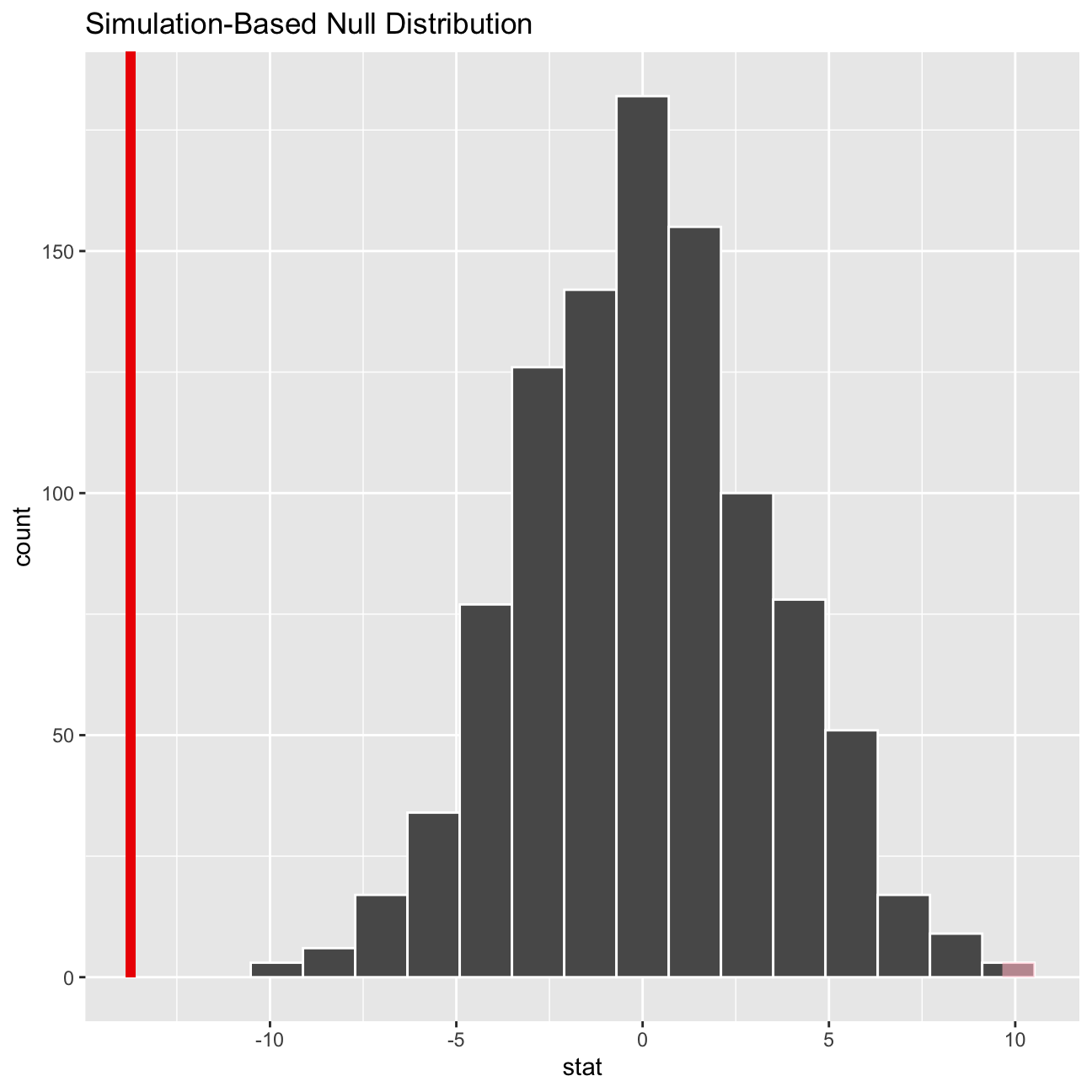
experience_null %>%
  get_p_value(obs_stat = obs_diff_eg, direction = "two_sided")
## # A tibble: 1 × 1
## p_value
## <dbl>
## 1 0Relationship between salary and experience?
To examine the relationship between salary and experience, a scatter plot is created.
ggplot(data = omega, aes(x = experience, y = salary, colour = gender)) +
  geom_point() +
  facet_wrap(~ gender) + # facet wrap
  theme_bw() +
  geom_smooth(se = FALSE) #no shade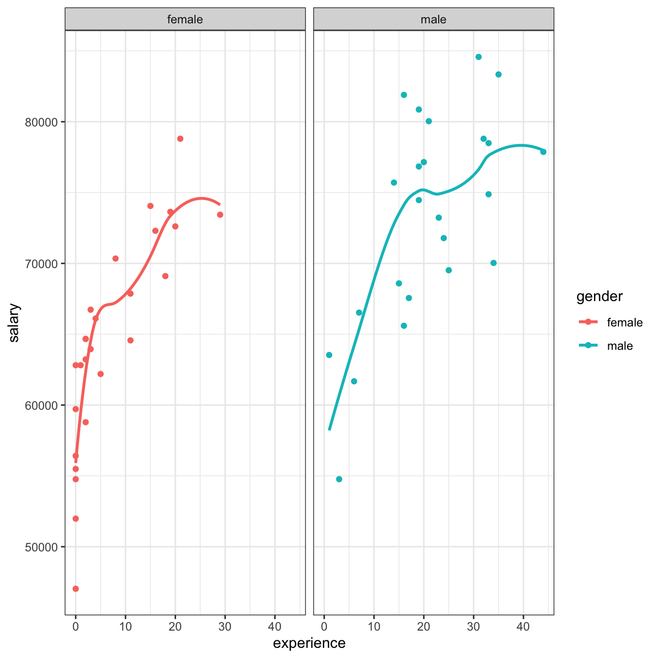
Check correlations between the data
Then, a scatter plot and a correlation matrix is created.
omega %>%
  select(gender, experience, salary) %>% #order variables they will appear in ggpairs()
  ggpairs(aes(colour=gender, alpha = 0.3))+
  theme_bw()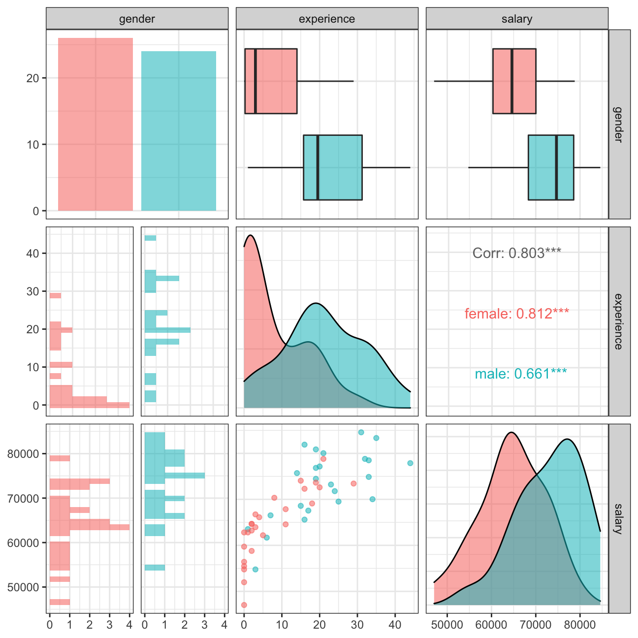
Looking at both plots, the correlation between salary and experience is stronger for females than males (0.812 vs 0.661). Therefore, on average, extra years of work experience have a greater impact on salary relative to their male counterparts. This is supported by the scatterplot. Moreover, there exists a pay gap between male and female.